Filter Examples
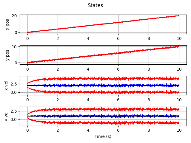
Kalman Filter
The Kalman filter can be setup using dynamic objects with the following.
 1def main():
 2    import numpy as np
 3    import numpy.random as rnd
 4    import matplotlib.pyplot as plt
 5
 6    import gncpy.plotting as gplot
 7    from gncpy.filters import KalmanFilter
 8    from gncpy.dynamics.basic import DoubleIntegrator
 9
10    # set measurement and process noise values
11    m_noise = 0.02
12    p_noise = 0.2
13    rng = rnd.default_rng(29)
14
15    # define the simulation time
16    dt = 0.01
17    t0, t1 = 0, 10
18    time = np.arange(t0, t1, dt)
19
20    # setup the filter
21    filt = KalmanFilter()
22    filt.cov = 0.25 * np.eye(4)
23
24    filt.set_state_model(dyn_obj=DoubleIntegrator())
25    filt.proc_noise = p_noise ** 2 * np.eye(4)
26
27    m_mat = np.array([[1, 0, 0, 0], [0, 1, 0, 0]])
28    filt.set_measurement_model(meas_mat=m_mat)
29    filt.meas_noise = m_noise ** 2 * np.eye(2)
30
31    # setup variables to save states and truth data
32    states = np.nan * np.ones((time.size, 4))
33    stds = np.nan * np.ones(states.shape)
34    states[0, :] = np.array([0, 0, 2, 1])
35    stds[0, :] = np.sqrt(np.diag(filt.cov))
36
37    t_states = states.copy()
38
39    # Run filter
40    A = DoubleIntegrator().get_state_mat(0, dt)
41    for kk, t in enumerate(time[:-1]):
42        states[kk + 1, :] = filt.predict(
43            t, states[kk, :].reshape((4, 1)), state_mat_args=(dt,)
44        ).flatten()
45        t_states[kk + 1, :] = (A @ t_states[kk, :].reshape((4, 1))).flatten()
46
47        n_state = m_mat @ (
48            t_states[kk + 1, :]
49            + np.sqrt(np.diag(filt.proc_noise)) * rng.standard_normal(1)
50        ).reshape((4, 1))
51        meas = n_state + m_noise * rng.standard_normal(n_state.size).reshape(
52            n_state.shape
53        )
54
55        states[kk + 1, :] = filt.correct(t, meas, states[kk + 1, :].reshape((4, 1)))[
56            0
57        ].flatten()
58        stds[kk + 1, :] = np.sqrt(np.diag(filt.cov))
59
60    # plot states
61    fig = plt.figure()
62    for ii, s in enumerate(DoubleIntegrator().state_names):
63        fig.add_subplot(4, 1, ii + 1)
64        fig.axes[ii].plot(time, states[:, ii], color="b", label="est")
65        fig.axes[ii].plot(time, t_states[:, ii], color="k", label="true")
66        fig.axes[ii].plot(time, states[:, ii] + stds[:, ii], color="r")
67        fig.axes[ii].plot(time, states[:, ii] - stds[:, ii], color="r")
68        fig.axes[ii].grid(True)
69        fig.axes[ii].set_ylabel(s)
70
71    plt_opts = gplot.init_plotting_opts()
72    gplot.set_title_label(fig, -1, plt_opts, ttl="States", x_lbl="Time (s)")
73    fig.tight_layout()
74
75    return fig
which gives this as output.
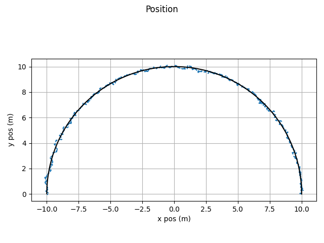
Extended Kalman Filter
The Extended Kalman filter can be setup using dynamic objects with the following.
 1def main():
 2    import numpy as np
 3    import numpy.random as rnd
 4    import matplotlib.pyplot as plt
 5
 6    import gncpy.plotting as gplot
 7    from gncpy.filters import ExtendedKalmanFilter
 8    from gncpy.dynamics.basic import CoordinatedTurnUnknown, CoordinatedTurnKnown
 9
10    d2r = np.pi / 180
11    r2d = 1 / d2r
12
13    # set measurement and process noise values
14    rng = rnd.default_rng(29)
15
16    p_posx_std = 0.2
17    p_posy_std = 0.2
18    p_velx_std = 0.3
19    p_vely_std = 0.3
20    p_turn_std = 0.2 * d2r
21
22    m_posx_std = 0.1
23    m_posy_std = 0.1
24
25    # create time vector
26    dt = 0.01
27    t0, t1 = 0, 10
28    time = np.arange(t0, t1, dt)
29
30    # create true dynamics object
31    trueDyn = CoordinatedTurnKnown(turn_rate=18 * d2r)
32
33    # create filter
34    coordTurn = CoordinatedTurnUnknown(dt=dt, turn_rate_cor_time=300)
35
36    filt = ExtendedKalmanFilter(cont_cov=True)
37    filt.cov = 0.5 ** 2 * np.eye(5)
38    filt.cov[4, 4] = (0.3 * d2r) ** 2
39
40    filt.set_state_model(dyn_obj=coordTurn)
41    filt.proc_noise = (
42        np.diag([p_posx_std, p_posy_std, p_velx_std, p_vely_std, p_turn_std]) ** 2
43    )
44
45    m_mat = np.array([[1, 0, 0, 0, 0], [0, 1, 0, 0, 0]])
46    filt.set_measurement_model(meas_mat=m_mat)
47    filt.meas_noise = np.diag([m_posx_std, m_posy_std]) ** 2
48
49    # set variables to save states
50    states = np.nan * np.ones((time.size, 5))
51    stds = np.nan * np.ones(states.shape)
52    stds[0, :] = np.sqrt(np.diag(filt.cov))
53    # set radius to be 10 m using v = omega r
54    states[0, :] = np.array([10, 0, 0, 10 * trueDyn.turn_rate, trueDyn.turn_rate])
55    t_states = states.copy()
56
57    Q = np.array([p_posx_std, p_posy_std, p_velx_std, p_vely_std, p_turn_std])
58    for kk, t in enumerate(time[:-1]):
59        # prediction
60        states[kk + 1, :] = filt.predict(t, states[kk, :].reshape((5, 1))).flatten()
61
62        # propagate truth and get measurement
63        t_states[kk + 1, :] = trueDyn.propagate_state(
64            t, t_states[kk, :].reshape((5, 1)), state_args=(dt,)
65        ).flatten()
66        meas = m_mat @ (t_states[kk + 1, :] + (Q * rng.standard_normal(5)))
67        meas += (
68            np.sqrt(np.diag(filt.meas_noise)) * rng.standard_normal(meas.size)
69        ).reshape(meas.shape)
70
71        # correction
72        states[kk + 1, :] = filt.correct(
73            t, meas.reshape((-1, 1)), states[kk + 1, :].reshape((5, 1))
74        )[0].ravel()
75        stds[kk + 1, :] = np.sqrt(np.diag(filt.cov))
76
77    # plot states
78    plt_opts = gplot.init_plotting_opts()
79    fig = plt.figure()
80    fig.add_subplot(1, 1, 1)
81    fig.axes[0].set_aspect("equal", adjustable="box")
82    fig.axes[0].plot(states[:, 0], states[:, 1], linestyle='--')
83    fig.axes[0].plot(
84        t_states[:, 0], t_states[:, 1], color="k", zorder=1000
85    )
86    fig.axes[0].grid(True)
87    gplot.set_title_label(
88        fig, 0, plt_opts, x_lbl="x pos (m)", y_lbl="y pos (m)", ttl="Position"
89    )
90    fig.tight_layout()
91
92    return fig
which gives this as output.
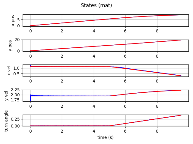
Interacting Multiple Model Filter
The Interacting Multiple Model filter can be setup using dynamic objects with the following.
  1def main():
  2    import numpy as np
  3    import numpy.random as rnd
  4    import matplotlib.pyplot as plt
  5
  6    import gncpy.plotting as gplot
  7    from gncpy.filters import KalmanFilter
  8    from gncpy.filters import InteractingMultipleModel
  9    from gncpy.dynamics.basic import CoordinatedTurnKnown
 10
 11    # set measurement and process noise values
 12    m_noise = 0.002
 13    p_noise = 0.004
 14
 15    dt = 0.01
 16    t0, t1 = 0, 9.5 + dt
 17    rng = rnd.default_rng(69)
 18
 19    dyn_obj1 = CoordinatedTurnKnown(turn_rate=0)
 20    dyn_obj2 = CoordinatedTurnKnown(turn_rate=5 * np.pi / 180)
 21
 22    in_filt1 = KalmanFilter()
 23    in_filt1.set_state_model(dyn_obj=dyn_obj1)
 24    m_mat = np.array([[1, 0, 0, 0, 0], [0, 1, 0, 0, 0], [0, 0, 0, 0, 1]])
 25    in_filt1.set_measurement_model(meas_mat=m_mat)
 26    in_filt1.cov = np.diag([0.25, 0.25, 3.0, 3.0, 0.25])
 27    gamma = np.array([0, 0, 1, 1, 0]).reshape((5, 1))
 28    # in_filt1.proc_noise = gamma @ np.array([[p_noise ** 2]]) @ gamma.T
 29    in_filt1.proc_noise = np.eye(5) * np.array([[p_noise ** 2]])
 30    in_filt1.meas_noise = m_noise ** 2 * np.eye(m_mat.shape[0])
 31
 32    in_filt2 = KalmanFilter()
 33    in_filt2.set_state_model(dyn_obj=dyn_obj2)
 34    in_filt2.set_measurement_model(meas_mat=m_mat)
 35    in_filt2.cov = np.diag([0.25, 0.25, 3.0, 3.0, 0.25])
 36    in_filt2.proc_noise = np.eye(5) * np.array([[p_noise ** 2]])
 37    # in_filt2.proc_noise = gamma @ np.array([[p_noise ** 2]]) @ gamma.T
 38    in_filt2.meas_noise = m_noise ** 2 * np.eye(m_mat.shape[0])
 39
 40    # vx0 = 2
 41    # vy0 = 1
 42    v = np.sqrt(2 ** 2 + 1 ** 2)
 43    angle = 60 * np.pi / 180
 44    vx0 = v * np.cos(angle)
 45    vy0 = v * np.sin(angle)
 46
 47    filt_list = [in_filt1, in_filt2]
 48
 49    model_trans = np.array([[1 - 1 / 200, 1 / 200], [1 / 200, 1 - 1 / 200]])
 50
 51    init_means = np.array([[0, 0, vx0, vy0, 0], [0, 0, vx0, vy0, 0]]).T
 52    init_covs = np.array([in_filt1.cov, in_filt2.cov])
 53
 54    filt = InteractingMultipleModel()
 55    filt.set_models(
 56        filt_list, model_trans, init_means, init_covs, init_weights=[0.5, 0.5]
 57    )
 58
 59    time = np.arange(t0, t1, dt)
 60    states = np.nan * np.ones((time.size, 5))
 61    stds = np.nan * np.ones(states.shape)
 62    pre_stds = stds.copy()
 63    states[0, :] = np.array([0, 0, vx0, vy0, 0])
 64    stds[0, :] = np.sqrt(np.diag(filt.cov))
 65    pre_stds[0, :] = stds[0, :]
 66
 67    t_states = states.copy()
 68
 69    for kk, t in enumerate(time[:-1]):
 70        states[kk + 1, :] = filt.predict(t, state_mat_args=(dt,)).flatten()
 71        if t < 5:
 72            t_states[kk + 1, :] = dyn_obj1.propagate_state(
 73                t, t_states[kk, :].reshape((5, 1)), state_args=(dt,)
 74            ).flatten()
 75        else:
 76            t_states[kk + 1, :] = dyn_obj2.propagate_state(
 77                t, t_states[kk, :].reshape((5, 1)), state_args=(dt,)
 78            ).flatten()
 79        pre_stds[kk + 1, :] = np.sqrt(np.diag(filt.cov))
 80
 81        n_state = m_mat @ (
 82            t_states[kk + 1, :].reshape((5, 1))
 83            + gamma * p_noise * rng.standard_normal(1)
 84        )
 85
 86        meas = (
 87            n_state + m_noise * rng.standard_normal(n_state.size).reshape(n_state.shape)
 88        ).reshape((-1, 1))
 89
 90        states[kk + 1, :] = filt.correct(t, meas)[0].flatten()
 91        stds[kk + 1, :] = np.sqrt(np.diag(filt.cov))
 92    errs = states - t_states
 93
 94# plot states
 95    fig = plt.figure()
 96    for ii, s in enumerate(CoordinatedTurnKnown().state_names):
 97        fig.add_subplot(5, 1, ii + 1)
 98        fig.axes[ii].plot(time, states[:, ii], color="b")
 99        fig.axes[ii].plot(time, t_states[:, ii], color="r")
100        fig.axes[ii].grid(True)
101        fig.axes[ii].set_ylabel(s)
102    fig.axes[-1].set_xlabel("time (s)")
103    fig.suptitle("States (mat)")
104    fig.tight_layout()
105
106    # # plot stds
107    # fig2 = plt.figure()
108    # for ii, s in enumerate(CoordinatedTurnKnown().state_names):
109    #     fig2.add_subplot(5, 1, ii + 1)
110    #     fig2.axes[ii].plot(time, stds[:, ii], color="b")
111    #     fig2.axes[ii].plot(time, np.abs(errs[:, ii]), color="r")
112    #     # fig.axes[ii].plot(time, pre_stds[:, ii], color="g")
113    #     fig2.axes[ii].grid(True)
114    #     fig2.axes[ii].set_ylabel(s + " std")
115    # fig2.axes[-1].set_xlabel("time (s)")
116    # fig2.suptitle("Filter standard deviations (mat)")
117    # fig2.tight_layout()
118    return fig
which gives this as output.