Control Examples
LQR Infinite Horizon Linear Dyanmics
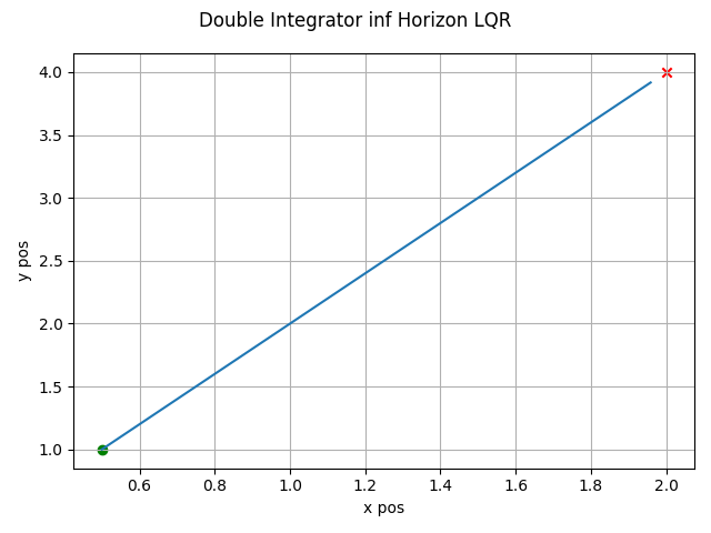
The LQR algorithm can be run for the infinite horizon case using linear dynamics with the following. Note the state trajectory output can be used as a motion plan.
 1def linear_inf_horizon():
 2    import numpy as np
 3
 4    import gncpy.dynamics.basic as gdyn
 5    from gncpy.control import LQR
 6
 7    cur_time = 0
 8    dt = 0.1
 9    cur_state = np.array([0.5, 1, 0, 0]).reshape((-1, 1))
10    end_state = np.array([2, 4, 0, 0]).reshape((-1, 1))
11    time_horizon = float("inf")
12
13    # Create dynamics object
14    dynObj = gdyn.DoubleIntegrator()
15    dynObj.control_model = lambda _t, *_args: np.array(
16        [[0, 0], [0, 0], [1, 0], [0, 1]]
17    )
18    state_args = (dt,)
19
20    # Setup LQR Object
21    u_nom = np.zeros((2, 1))
22    Q = 10 * np.eye(len(dynObj.state_names))
23    R = 0.5 * np.eye(u_nom.size)
24    lqr = LQR(time_horizon=time_horizon)
25    # need to set dt here so the controller can generate a state trajectory
26    lqr.set_state_model(u_nom, dynObj=dynObj, dt=dt)
27    lqr.set_cost_model(Q, R)
28
29    u, cost, state_traj, ctrl_signal = lqr.calculate_control(
30        cur_time,
31        cur_state,
32        end_state=end_state,
33        end_state_tol=0.1,
34        check_inds=[0, 1],
35        state_args=state_args,
36        provide_details=True,
37    )
38
39    return state_traj, end_state
which gives this as output.
LQR Finite Horzon Linear Dynamics
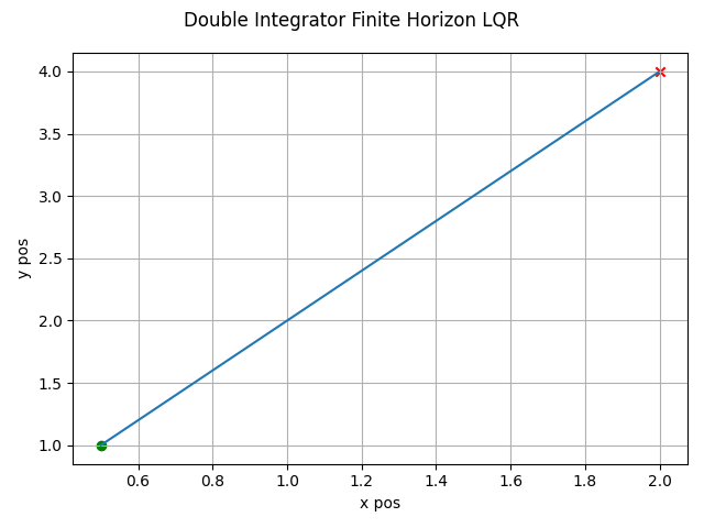
The LQR algorithm can be run for the finite horizon case using non-linear dynamics with the following. Note the state trajectory output can be used as a motion plan.
 1def linear_finite_horizon():
 2    import numpy as np
 3
 4    import gncpy.dynamics.basic as gdyn
 5    from gncpy.control import LQR
 6
 7    cur_time = 0
 8    dt = 0.1
 9    cur_state = np.array([0.5, 1, 0, 0]).reshape((-1, 1))
10    end_state = np.array([2, 4, 0, 0]).reshape((-1, 1))
11    time_horizon = 3 * dt
12
13    # Create dynamics object
14    dynObj = gdyn.DoubleIntegrator()
15    dynObj.control_model = lambda _t, *_args: np.array(
16        [[0, 0], [0, 0], [1, 0], [0, 1]]
17    )
18    state_args = (dt,)
19    inv_state_args = (-dt, )
20
21    # Setup LQR Object
22    u_nom = np.zeros((2, 1))
23    Q = 200 * np.eye(len(dynObj.state_names))
24    R = 0.01 * np.eye(u_nom.size)
25    lqr = LQR(time_horizon=time_horizon)
26    # need to set dt here so the controller can generate a state trajectory
27    lqr.set_state_model(u_nom, dynObj=dynObj, dt=dt)
28    lqr.set_cost_model(Q, R)
29
30    u, cost, state_traj, ctrl_signal = lqr.calculate_control(
31        cur_time,
32        cur_state,
33        end_state=end_state,
34        state_args=state_args,
35        inv_state_args=inv_state_args,
36        provide_details=True,
37    )
38
39    return state_traj, end_state
which gives this as output.
LQR Finite Horzon Non-linear Dynamics
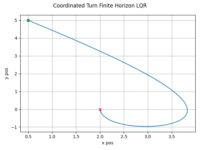
The LQR algorithm can be run for the finite horizon case using non-linear dynamics with the following. Note the state trajectory output can be used as a motion plan.
 1def nonlin_finite_hor():
 2    import numpy as np
 3
 4    import gncpy.dynamics.basic as gdyn
 5    from gncpy.control import LQR
 6
 7    d2r = np.pi / 180
 8
 9    cur_time = 0
10    dt = 0.1
11    cur_state = np.array([0.5, 0, 5, 45 * d2r]).reshape((-1, 1))
12    end_state = np.array([2, 0, 0, 0]).reshape((-1, 1))
13    time_horizon = 50 * dt
14
15    # Create dynamics object
16    dynObj = gdyn.CurvilinearMotion()
17
18    # Setup LQR Object
19    u_nom = np.zeros((2, 1))
20    Q = np.diag([200, 2000, 200, 2000])
21    R = 0.01 * np.eye(u_nom.size)
22    lqr = LQR(time_horizon=time_horizon)
23    # need to set dt here so the controller can generate a state trajectory
24    lqr.set_state_model(u_nom, dynObj=dynObj, dt=dt)
25    lqr.set_cost_model(Q, R)
26
27    u, cost, state_traj, ctrl_signal = lqr.calculate_control(
28        cur_time,
29        cur_state,
30        end_state=end_state,
31        provide_details=True,
32    )
33
34    return state_traj, end_state
which gives this as output.
ELQR
The ELQR algorithm can be run for a finite horizon with non-linear dynamics and a non-quadratic cost with the following. Note the state trajectory output can be used as a motion plan. This version does not modify the quadratization process.
  1def basic():
  2    import numpy as np
  3
  4    import gncpy.plotting as gplot
  5    import gncpy.control as gctrl
  6    from gncpy.dynamics.basic import IRobotCreate
  7
  8    tt = 0  # starting time when calculating control
  9    dt = 1 / 6
 10    time_horizon = 150 * dt  # run for 150 timesteps
 11
 12    # define starting and ending state for control calculation
 13    end_state = np.array([0, 2.5, np.pi]).reshape((3, 1))
 14    start_state = np.array([0, -2.5, np.pi]).reshape((3, 1))
 15
 16    # define nominal control input
 17    u_nom = np.zeros((2, 1))
 18
 19    # define dynamics
 20    # IRobot Create has a dt that can be set here or it can be set by the control
 21    # algorithm
 22    dynObj = IRobotCreate(wheel_separation=0.258, radius=0.335 / 2.0)
 23
 24    # define some circular obstacles with center pos and radius (x, y, radius)
 25    obstacles = np.array(
 26        [
 27            [0, -1.35, 0.2],
 28            [1.0, -0.5, 0.2],
 29            [-0.95, -0.5, 0.2],
 30            [-0.2, 0.3, 0.2],
 31            [0.8, 0.7, 0.2],
 32            [1.1, 2.0, 0.2],
 33            [-1.2, 0.8, 0.2],
 34            [-1.1, 2.1, 0.2],
 35            [-0.1, 1.6, 0.2],
 36            [-1.1, -1.9, 0.2],
 37            [(10 + np.sqrt(2)) / 10, (-15 - np.sqrt(2)) / 10, 0.2],
 38        ]
 39    )
 40
 41    # define enviornment bounds for the robot
 42    bottom_left = np.array([-2, -3])
 43    top_right = np.array([2, 3])
 44
 45    # define Q and R weights for using standard cost function
 46    # Q = np.diag([50, 50, 0.4 * np.pi / 2])
 47    Q = 50 * np.eye(3)
 48    R = 0.6 * np.eye(u_nom.size)
 49
 50    # define non-quadratic term for cost function
 51    # has form: (tt, state, ctrl_input, end_state, is_initial, is_final, *args)
 52    obs_factor = 1
 53    scale_factor = 1
 54    cost_args = (obstacles, obs_factor, scale_factor, bottom_left, top_right)
 55
 56    def non_quadratic_cost(
 57        tt,
 58        state,
 59        ctrl_input,
 60        end_state,
 61        is_initial,
 62        is_final,
 63        _obstacles,
 64        _obs_factor,
 65        _scale_factor,
 66        _bottom_left,
 67        _top_right,
 68    ):
 69        cost = 0
 70        # cost for obstacles
 71        for obs in _obstacles:
 72            diff = state.ravel()[0:2] - obs[0:2]
 73            dist = np.sqrt(np.sum(diff * diff))
 74            # signed distance is negative if the robot is within the obstacle
 75            signed_dist = (dist - dynObj.radius) - obs[2]
 76            if signed_dist > 0:
 77                continue
 78            cost += _obs_factor * np.exp(-_scale_factor * signed_dist).item()
 79
 80        # add cost for going out of bounds
 81        for ii, b in enumerate(_bottom_left):
 82            dist = (state[ii] - b) - dynObj.radius
 83            cost += _obs_factor * np.exp(-_scale_factor * dist).item()
 84
 85        for ii, b in enumerate(_top_right):
 86            dist = (b - state[ii]) - dynObj.radius
 87            cost += _obs_factor * np.exp(-_scale_factor * dist).item()
 88
 89        return cost
 90
 91    # create control obect
 92    elqr = gctrl.ELQR(time_horizon=time_horizon)
 93    elqr.set_state_model(u_nom, dynObj=dynObj)
 94    elqr.dt = dt  # set here or within the dynamic object
 95    elqr.set_cost_model(Q=Q, R=R, non_quadratic_fun=non_quadratic_cost)
 96
 97    # create figure with obstacles to plot animation on
 98    fig = plt.figure()
 99    fig.add_subplot(1, 1, 1)
100    fig.axes[0].set_aspect("equal", adjustable="box")
101    fig.axes[0].set_xlim((bottom_left[0], top_right[0]))
102    fig.axes[0].set_ylim((bottom_left[1], top_right[1]))
103    fig.axes[0].scatter(
104        start_state[0], start_state[1], marker="o", color="g", zorder=1000
105    )
106    for obs in obstacles:
107        c = Circle(obs[:2], radius=obs[2], color="k", zorder=1000)
108        fig.axes[0].add_patch(c)
109    plt_opts = gplot.init_plotting_opts(f_hndl=fig)
110    gplot.set_title_label(fig, 0, plt_opts, ttl="ELQR")
111
112    # calculate control
113    u, cost, state_trajectory, control_signal, fig, frame_list = elqr.calculate_control(
114        tt,
115        start_state,
116        end_state,
117        cost_args=cost_args,
118        provide_details=True,
119        show_animation=True,
120        save_animation=True,
121        plt_inds=[0, 1],
122        fig=fig,
123    )
124
125    return frame_list
which gives this as output.
ELQR Modified Quadratization
The ELQR algorithm can be run for a finite horizon with non-linear dynamics and a non-quadratic cost with the following. Note the state trajectory output can be used as a motion plan. This version does modifies the quadratization process.
  1def modify_quadratize():
  2    import numpy as np
  3
  4    import gncpy.plotting as gplot
  5    import gncpy.control as gctrl
  6    from gncpy.dynamics.basic import IRobotCreate
  7
  8    tt = 0  # starting time when calculating control
  9    dt = 1 / 6
 10    time_horizon = 150 * dt  # run for 150 timesteps
 11
 12    # define starting and ending state for control calculation
 13    end_state = np.array([0, 2.5, np.pi]).reshape((3, 1))
 14    start_state = np.array([0, -2.5, np.pi]).reshape((3, 1))
 15
 16    # define nominal control input
 17    u_nom = np.zeros((2, 1))
 18
 19    # define dynamics
 20    # IRobot Create has a dt that can be set here or it can be set by the control
 21    # algorithm
 22    dynObj = IRobotCreate(wheel_separation=0.258, radius=0.335 / 2.0)
 23
 24    # define some circular obstacles with center pos and radius (x, y, radius)
 25    obstacles = np.array(
 26        [
 27            [0, -1.35, 0.2],
 28            [1.0, -0.5, 0.2],
 29            [-0.95, -0.5, 0.2],
 30            [-0.2, 0.3, 0.2],
 31            [0.8, 0.7, 0.2],
 32            [1.1, 2.0, 0.2],
 33            [-1.2, 0.8, 0.2],
 34            [-1.1, 2.1, 0.2],
 35            [-0.1, 1.6, 0.2],
 36            [-1.1, -1.9, 0.2],
 37            [(10 + np.sqrt(2)) / 10, (-15 - np.sqrt(2)) / 10, 0.2],
 38        ]
 39    )
 40
 41    # define enviornment bounds for the robot
 42    bottom_left = np.array([-2, -3])
 43    top_right = np.array([2, 3])
 44
 45    # define Q and R weights for using standard cost function
 46    Q = 50 * np.eye(len(dynObj.state_names))
 47    R = 0.6 * np.eye(u_nom.size)
 48
 49    # define non-quadratic term for cost function
 50    # has form: (tt, state, ctrl_input, end_state, is_initial, is_final, *args)
 51    obs_factor = 1
 52    scale_factor = 1
 53    cost_args = (obstacles, obs_factor, scale_factor, bottom_left, top_right)
 54
 55    def non_quadratic_cost(
 56        tt,
 57        state,
 58        ctrl_input,
 59        end_state,
 60        is_initial,
 61        is_final,
 62        _obstacles,
 63        _obs_factor,
 64        _scale_factor,
 65        _bottom_left,
 66        _top_right,
 67    ):
 68        cost = 0
 69        # cost for obstacles
 70        for obs in _obstacles:
 71            diff = state.ravel()[0:2] - obs[0:2]
 72            dist = np.sqrt(np.sum(diff * diff))
 73            # signed distance is negative if the robot is within the obstacle
 74            signed_dist = (dist - dynObj.radius) - obs[2]
 75            if signed_dist > 0:
 76                continue
 77            cost += _obs_factor * np.exp(-_scale_factor * signed_dist).item()
 78
 79        # add cost for going out of bounds
 80        for ii, b in enumerate(_bottom_left):
 81            dist = (state[ii] - b) - dynObj.radius
 82            cost += _obs_factor * np.exp(-_scale_factor * dist).item()
 83
 84        for ii, b in enumerate(_top_right):
 85            dist = (b - state[ii]) - dynObj.radius
 86            cost += _obs_factor * np.exp(-_scale_factor * dist).item()
 87
 88        return cost
 89
 90    # define modifications for quadratizing the cost function
 91    def quad_modifier(itr, tt, P, Q, R, q, r):
 92        rot_cost = 0.4
 93        # only modify if within the first 2 iterations
 94        if itr < 2:
 95            Q[-1, -1] = rot_cost
 96            q[-1] = -rot_cost * np.pi / 2
 97
 98        return P, Q, R, q, r
 99
100    # create control obect
101    elqr = gctrl.ELQR(time_horizon=time_horizon)
102    elqr.set_state_model(u_nom, dynObj=dynObj)
103    elqr.dt = dt  # set here or within the dynamic object
104    elqr.set_cost_model(
105        Q=Q, R=R, non_quadratic_fun=non_quadratic_cost, quad_modifier=quad_modifier
106    )
107
108    fig = plt.figure()
109    fig.add_subplot(1, 1, 1)
110    fig.axes[0].set_aspect("equal", adjustable="box")
111    fig.axes[0].set_xlim((bottom_left[0], top_right[0]))
112    fig.axes[0].set_ylim((bottom_left[1], top_right[1]))
113    fig.axes[0].scatter(
114        start_state[0], start_state[1], marker="o", color="g", zorder=1000
115    )
116    for obs in obstacles:
117        c = Circle(obs[:2], radius=obs[2], color="k", zorder=1000)
118        fig.axes[0].add_patch(c)
119    plt_opts = gplot.init_plotting_opts(f_hndl=fig)
120    gplot.set_title_label(fig, 0, plt_opts, ttl="ELQR with Modified Quadratize Cost")
121
122    # calculate control
123    u, cost, state_trajectory, control_signal, fig, frame_list = elqr.calculate_control(
124        tt,
125        start_state,
126        end_state,
127        cost_args=cost_args,
128        provide_details=True,
129        show_animation=True,
130        save_animation=True,
131        plt_inds=[0, 1],
132        fig=fig,
133    )
134
135    return frame_list
which gives this as output.
ELQR Linear Dynamics
The ELQR algorithm can be run for a finite horizon with linear dynamics and a non-quadratic cost with the following. Note the state trajectory output can be used as a motion plan. This version uses dynamics with a constraint on the states in addition to the obstacles in the environment.
  1def linear():
  2    import numpy as np
  3
  4    import gncpy.plotting as gplot
  5    import gncpy.control as gctrl
  6    from gncpy.dynamics.basic import DoubleIntegrator
  7
  8    tt = 0  # starting time when calculating control
  9    dt = 1 / 6
 10    time_horizon = 20 * dt  # run for 150 timesteps
 11
 12    # define starting and ending state for control calculation
 13    end_state = np.array([0, 2.5, 0, 0]).reshape((-1, 1))
 14    start_state = np.array([0, -2.5, 0, 0]).reshape((-1, 1))
 15
 16    # define nominal control input
 17    u_nom = np.zeros((2, 1))
 18
 19    # define dynamics
 20    dynObj = DoubleIntegrator()
 21
 22    # set control model
 23    dynObj.control_model = lambda t, *args: np.array(
 24        [[0, 0], [0, 0], [1, 0], [0, 1]], dtype=float
 25    )
 26
 27    # set a state constraint on the velocities
 28    dynObj.state_constraint = lambda t, x: np.vstack(
 29        (
 30            x[:2],
 31            np.max(
 32                (np.min((x[2:], 2 * np.ones((2, 1))), axis=0), -2 * np.ones((2, 1))),
 33                axis=0,
 34            ),
 35        )
 36    )
 37
 38    # define some circular obstacles with center pos and radius (x, y, radius)
 39    obstacles = np.array(
 40        [
 41            [0, -1.35, 0.2],
 42            [1.0, -0.5, 0.2],
 43            [-0.95, -0.5, 0.2],
 44            [-0.2, 0.3, 0.2],
 45            [0.8, 0.7, 0.2],
 46            [1.1, 2.0, 0.2],
 47            [-1.2, 0.8, 0.2],
 48            [-1.1, 2.1, 0.2],
 49            [-0.1, 1.6, 0.2],
 50            [-1.1, -1.9, 0.2],
 51            [(10 + np.sqrt(2)) / 10, (-15 - np.sqrt(2)) / 10, 0.2],
 52        ]
 53    )
 54
 55    # define enviornment bounds for the robot
 56    bottom_left = np.array([-2, -3])
 57    top_right = np.array([2, 3])
 58
 59    # define Q and R weights for using standard cost function
 60    Q = 10 * np.eye(len(dynObj.state_names))
 61    R = 0.6 * np.eye(u_nom.size)
 62
 63    # define non-quadratic term for cost function
 64    # has form: (tt, state, ctrl_input, end_state, is_initial, is_final, *args)
 65    obs_factor = 1
 66    scale_factor = 1
 67    cost_args = (obstacles, obs_factor, scale_factor, bottom_left, top_right)
 68
 69    def non_quadratic_cost(
 70        tt,
 71        state,
 72        ctrl_input,
 73        end_state,
 74        is_initial,
 75        is_final,
 76        _obstacles,
 77        _obs_factor,
 78        _scale_factor,
 79        _bottom_left,
 80        _top_right,
 81    ):
 82        cost = 0
 83        radius = 0.335 / 2.0
 84        # cost for obstacles
 85        for obs in _obstacles:
 86            diff = state.ravel()[0:2] - obs[0:2]
 87            dist = np.sqrt(np.sum(diff * diff))
 88            # signed distance is negative if the robot is within the obstacle
 89            signed_dist = (dist - radius) - obs[2]
 90            if signed_dist > 0:
 91                continue
 92            cost += _obs_factor * np.exp(-_scale_factor * signed_dist).item()
 93
 94        # add cost for going out of bounds
 95        for ii, b in enumerate(_bottom_left):
 96            dist = (state[ii] - b) - radius
 97            cost += _obs_factor * np.exp(-_scale_factor * dist).item()
 98
 99        for ii, b in enumerate(_top_right):
100            dist = (b - state[ii]) - radius
101            cost += _obs_factor * np.exp(-_scale_factor * dist).item()
102
103        return cost
104
105    # create control obect
106    elqr = gctrl.ELQR(time_horizon=time_horizon)
107    elqr.set_state_model(u_nom, dynObj=dynObj)
108    elqr.dt = dt  # set here or within the dynamic object
109    elqr.set_cost_model(Q=Q, R=R, non_quadratic_fun=non_quadratic_cost)
110
111    fig = plt.figure()
112    fig.add_subplot(1, 1, 1)
113    fig.axes[0].set_aspect("equal", adjustable="box")
114    fig.axes[0].set_xlim((bottom_left[0], top_right[0]))
115    fig.axes[0].set_ylim((bottom_left[1], top_right[1]))
116    fig.axes[0].scatter(
117        start_state[0], start_state[1], marker="o", color="g", zorder=1000
118    )
119    for obs in obstacles:
120        c = Circle(obs[:2], radius=obs[2], color="k", zorder=1000)
121        fig.axes[0].add_patch(c)
122    plt_opts = gplot.init_plotting_opts(f_hndl=fig)
123    gplot.set_title_label(fig, 0, plt_opts, ttl="ELQR with Linear Dynamics Cost")
124
125    # calculate control
126    u, cost, state_trajectory, control_signal, fig, frame_list = elqr.calculate_control(
127        tt,
128        start_state,
129        end_state,
130        state_args=(dt,),
131        cost_args=cost_args,
132        inv_state_args=(-dt,),
133        provide_details=True,
134        show_animation=True,
135        save_animation=True,
136        plt_inds=[0, 1],
137        fig=fig,
138    )
139
140    return frame_list
which gives this as output.