Data Fusion Examples

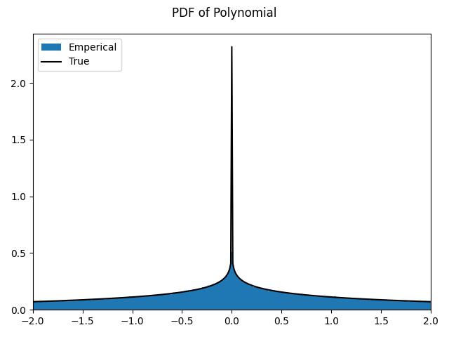
Gaussian Multiplication

The PDF of the multiplication of two zero mean normal PDFs follows a Normal Product distribution see here. For random variables \(X, Y\) with zero mean and standard deviations \(\sigma_X, \sigma_Y\) the product of their PDF follows the PDF given by

\[P_{X,Y}(u) = \frac{K_0(\frac{\vert u \vert}{\sigma_X\sigma_Y})}{\pi\sigma_X\sigma_Y}\]

where \(K_0(z)\) is the modified Bessel function of the second kind.

def multiplication():
    import scipy.special
    import numpy as np
    import matplotlib.pyplot as plt

    from serums.distribution_overbounder import fusion
    from serums.models import Gaussian

    std_x = np.sqrt(4)
    std_y = np.sqrt(6)

    x = Gaussian(mean=np.array([[0]]), covariance=np.array([[std_x**2]]))
    y = Gaussian(mean=np.array([[0]]), covariance=np.array([[std_y**2]]))
    x.monte_carlo_size = 1e6

    poly = lambda x_, y_: x_ * y_

    z = fusion([x, y], poly)

    plt_x_bnds = (-2, 2)
    pts = np.arange(*plt_x_bnds, 0.01)
    true_pdf = scipy.special.kn(0, np.abs(pts) / (std_x * std_y)) / (
        np.pi * std_x * std_y
    )

    fig = plt.figure()
    fig.add_subplot(1, 1, 1)
    fig.axes[0].hist(
        z,
        density=True,
        bins=int(1e4),
        histtype="stepfilled",
        label="Emperical",
    )
    fig.axes[0].plot(pts, true_pdf, label="True", color="k", zorder=1000)
    fig.axes[0].legend(loc="upper left")
    fig.suptitle("PDF of Polynomial")
    fig.axes[0].set_xlim(plt_x_bnds)
    fig.tight_layout()

    return fig

The above script gives this as output.

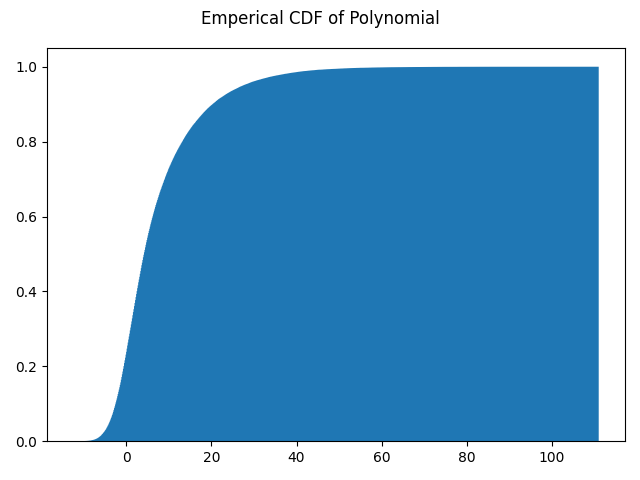
General Polynomial

Data fusion for a generic polynomial function can be performed as shown in the following script. Note Gaussians are used here as an example however, any child of serums.models.BaseSingleModel can be used.

def main():
    import numpy as np
    import matplotlib.pyplot as plt

    from serums.distribution_overbounder import fusion
    from serums.models import Gaussian

    x = Gaussian(mean=np.array([[2]]), covariance=np.array([[4]]))
    y = Gaussian(mean=np.array([[-3]]), covariance=np.array([[6]]))
    x.monte_carlo_size = 1e5

    poly = lambda x_, y_: x_ + y_ + x_**2

    z = fusion([x, y], poly)

    fig = plt.figure()
    fig.add_subplot(1, 1, 1)
    fig.axes[0].hist(z, density=True, cumulative=True, bins=1000, histtype="stepfilled")
    fig.suptitle("Emperical CDF of Polynomial")
    fig.tight_layout()

    return fig

The above script gives this as output.

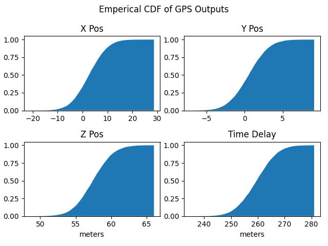
GPS Examples

An example of a real world application is GPS pseudorange measurements. Here it is assumed the reciever and satellite positions are known but the measured pseudoranges follow a Gaussian distribution. This is based on [7]. Note, a Gaussian is used for simplicity but any child of serums.models.BaseSingleModel may be used. The following script shows how to get samples from the fused distribution for output position and time delay. These outputs are often what is of interest instead of the measured pseudoranges. A linearized transformation from pseudoranges to positions is used.

def main():
    import numpy as np
    import matplotlib.pyplot as plt
    from numpy.linalg import inv

    from serums.distribution_overbounder import fusion
    from serums.models import Gaussian

    # assume that user position and gps SV positions are known
    user_pos = np.array([-41.772709, -16.789194, 6370.059559, 999.76252931])
    gps_pos_lst = np.array(
        [
            [15600, 7540, 20140],
            [18760, 2750, 18610],
            [17610, 14630, 13480],
            [19170, 610, 18390],
        ],
        dtype=float,
    )

    # define the noise on each pseudorange as a Gaussian (assume the same covariance for simplicity)
    std_pr = 10
    pr_means = np.sqrt(np.sum((gps_pos_lst - user_pos[:3]) ** 2, axis=1))
    prs = []
    for m in pr_means:
        prs.append(
            Gaussian(
                mean=m.reshape((-1, 1)).copy(), covariance=np.array([[std_pr**2]])
            )
        )

    # define the uncertainty matrix
    R = np.diag(std_pr * np.ones(len(prs)))

    # create the linearized GPS measurement matrix with a function
    def make_G(user_pos_: np.ndarray) -> np.ndarray:
        G = None
        for ii, sv_pos in enumerate(gps_pos_lst):
            diff = user_pos_.ravel()[:3] - sv_pos
            row = np.hstack((diff / np.sqrt(np.sum(diff**2)), np.array([1])))
            if G is None:
                G = row
            else:
                G = np.vstack((G, row))
        return G

    # define the mapping matrix (this will be used in the polynomial)
    G = make_G(user_pos)
    S = inv(G.T @ R @ G) @ G.T @ inv(R)

    fig = plt.figure()
    [fig.add_subplot(2, 2, ii + 1) for ii in range(4)]
    fig.suptitle("Emperical CDF of GPS Outputs")
    ttl_lst = ["X Pos", "Y Pos", "Z Pos", "Time Delay"]

    # define the fusion polynomial for each output variable (ie x/y/z pos and time delay)
    for ii, ttl in enumerate(ttl_lst):
        poly = (
            lambda pr0, pr1, pr2, pr3: S[ii, 0] * pr0
            + S[ii, 1] * pr1
            + S[ii, 2] * pr2
            + S[ii, 3] * pr3
        )
        # these samples could then be run through an overbounding routine
        samples = fusion(prs, poly)

        # plot the emperical CDF to view results
        fig.axes[ii].hist(
            samples,
            density=True,
            cumulative=True,
            bins=int(1e3),
            histtype="stepfilled",
        )
        fig.axes[ii].set_title(ttl)
        if ii == 2 or ii == 3:
            fig.axes[ii].set_xlabel("meters")

    fig.tight_layout()

    return fig

The above script gives this as output.